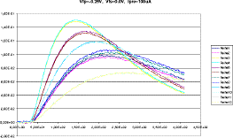
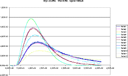
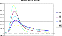
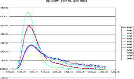
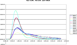
The relation between the curve labeled "Reihe 1" ... "Reihe 12" is given in the following table:
| Reihe 1 | 29.4pF |
| Reihe 2 | 29.4pF |
| Reihe 3 | 0pF |
| Reihe 4 | 0pF |
| Reihe 5 | 6.8pF |
| Reihe 6 | 6.8pF |
| Reihe 7 | 29.4pF |
| Reihe 8 | 29.4pF |
| Reihe 9 | 16.3pF |
| Reihe 10 | 16.3pF |
| Reihe 11 | 58pF |
| Reihe 12 | 58pF |
The y-Axis is the measured amplitude in V with an analogue receiver circuit as described in the Helix128-x User manual at the section "The analog receiver circuit" with a feedback resistance of 300Ohms.
The preview links to a Postscript file containing the plot. The text
header in each table cell links to an ASCII data file which contains the
pulse shape data. Data in this file is organized in columns. The first
column contains the time, the other columns contain the pulse shape amplitude.
| Ipre=100uA | |
|---|---|
| Vfs=0.0V |
|
| Vfs=0.5V |
|
| Vfs=1.0V |
|
| Vfs=1.5V |
|
| Vfs=2.0V |
|
Last changes: 99/11/12 by Martin Feuerstack-Raible
If you have comments or suggestions, email Ulrich Trunk